A Transferable Climate Profile Framework
Using WorldClim v2.1 and CMIP6 SSP Projections
Case Study: Cambodia

Version 2

Author

Richard T. Cooper

Published

October 13, 2026

Introduction

A climate profile is an essential element of any climate risk assessment, as it provides the quantitative baseline and future projections necessary to identify climate hazards, evaluate exposure, and inform adaptation planning. This climate profile is part of a larger framework under development for assessing climate risk, which will be shared once completed.

This Quarto document provides a transparent, reproducible and transferable framework for generating a set of key maps and graphs required for a climate profile. Outputs are based on the WorldClim 2.1 climate dataset, including historical (1970–2000) and CMIP6 projected data for two future periods (2041–2060 and 2061–2080) under two shared socioeconomic pathways (SSP): SSP2-4.5 (moderate) and SSP5-8.5 (very high) emission scenarios. Future projections for Cambodia are based on an ensemble of five global climate models (GCMs)—ACCESS-CM2, MIROC6, EC-Earth3-Veg, MRI-ESM2-0, and IPSL-CM6A-LR. While demonstrated here at the national level, the boundary used to crop data inputs can be readily adjusted to any administrative region or river basin boundary, making the script adaptable to sub-national and watershed-level climate assessments.

WorldClim is a popular open-source climate dataset, recognised for its global coverage and fine spatial resolution (1 km). However, as data are provided as monthly means, they cannot support derivation of daily-based climate change indices, such as heavy precipitation frequency, the number of consecutive dry days, or percentile-based metrics (e.g., as defined by the ETCCDI).¹ Daily-based climate change indices could be generated by downscaling NASA NEX-GDDP-CMIP6 datasets with CHELSA-W5E5.²

The climate profile outputs are organised into three sections. The first two use only WorldClim monthly variables and can be reproduced for any country: the historical baseline (1970–2000) and future projections under SSP2-4.5 and SSP5-8.5. The third is tailored to the region and sector of interest, in this case Cambodia and rice farming, and is structured around the country’s monsoonal wet season (May–November) and dry season (December–April) (Chhinh & Millington, 2015).

The historical baseline is presented through maps of mean annual temperature and mean annual precipitation, and a climate chart of mean monthly precipitation and temperature.

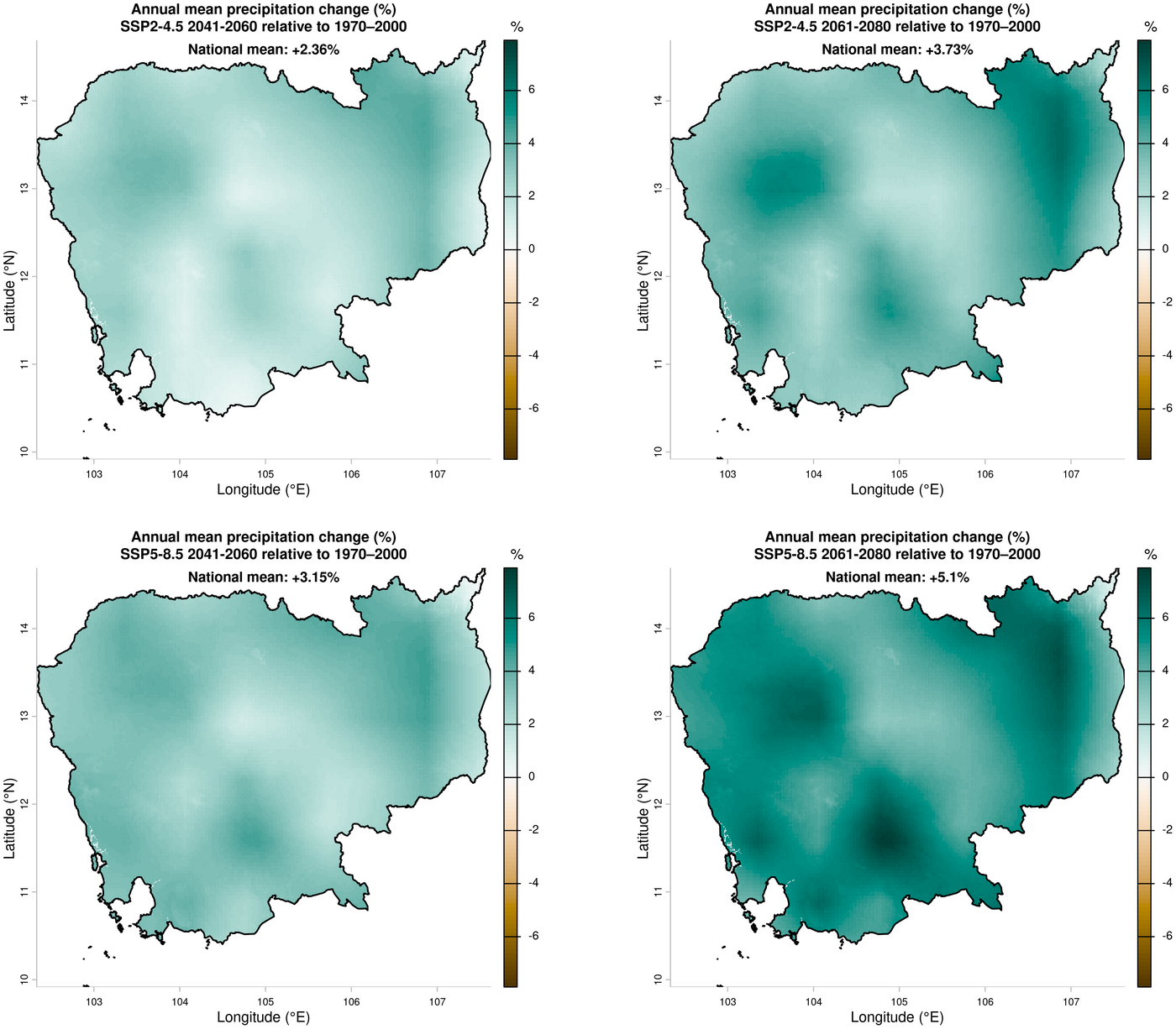
Future projections for 2041–2060 and 2061–2080 are presented through three complementary visualisations: spatial anomaly panel maps of mean annual temperature and precipitation change; model ensemble spread plots of mean annual temperature and precipitation anomalies across the five GCMs; and ensemble range plots of mean monthly temperature and precipitation with GCM uncertainty envelopes.

The region- and sector-specific outputs comprise spatial anomaly panel maps of wet-season and dry-season precipitation change and of dry-season mean temperature change; a monthly precipitation ensemble range plot overlaid with the wet and dry seasons and the onset and cessation of the south-west monsoon; and a mean monthly maximum temperature ensemble range plot against a 35 °C threshold, an indicative level for heat stress in rice.

Prerequisites

Install and load R packages.

## Install R packages
#
# Installs the latest stable R package versions from the CRAN repository.
# Safe to run every time: packages already installed are skipped.
#
# On Ubuntu, may need to install these operating system packages first:
# sudo apt-get install libabsl-dev cmake
# magick also needs the ImageMagick development libraries:
# sudo apt-get install libmagick++-dev

# Alternative: latest development code from GitHub (remotes::install_github)
# if (!require(remotes)) {
#   install.packages("remotes")
# }
# library(remotes)
#
# if (!require(terra)) {
#   remotes::install_github("rspatial/terra")
# }

options(repos = c(CRAN = "https://cloud.r-project.org"))

# terra installed first and separately — it has system-level
# GDAL/GEOS/PROJ dependencies, so isolating it here gives a clearer
# error message if it fails.
if (!require(terra)) {
  install.packages("terra")
}

# Everything else used in this document.
required_packages <- c(
  "codetools",  # address terra error message
  "geodata",    # WorldClim/CMIP6 downloads, GADM boundaries
  "magick"      # combine and annotate map images
)

# Go through each required package one at a time, checking whether it's
# already installed. Anything not found gets added to a growing list of
# packages still needed.
missing_packages <- c()
for (pkg in required_packages) {
  if (!requireNamespace(pkg, quietly = TRUE)) {
    missing_packages <- c(missing_packages, pkg)
  }
}

if (length(missing_packages) > 0) {
  message("Installing missing packages: ", paste(missing_packages, collapse = ", "))
  install.packages(missing_packages)
} else {
  message("All required packages already installed.")
}

## Load libraries
library(terra)
library(codetools)
library(geodata)
library(magick)

Download GCM data: five models, two scenarios and two future periods

The selection of models used is based on a preliminary review of literature pertinent to the case study area of Cambodia.

# Modify with country ISO code (used to download country boundary)
country_iso <- "KHM"

# Specify lat and lon of area of WorldClim data to be downloaded
lat <- 8
lon <- 100

gcms <-
  c(
    "ACCESS-CM2",
    "MIROC6",
    "EC-Earth3-Veg",
    "MRI-ESM2-0",
    "IPSL-CM6A-LR"
  )
ssps <- c("245", "585")
years <- c("2041-2060", "2061-2080")
vars <- c("tmin", "tmax", "prec")

# Season definition: Cambodia's monsoonal system — dry season Dec-Apr,
# wet season May-Nov (per Chhinh & Millington, 2015).
wet_months <- 5:11
dry_months <- c(12, 1, 2, 3, 4)

# Directories to store WorldClim data — named by country_iso, so re-running
# for a different country automatically uses a separate folder.
out_dir <- paste0("wc_downloads_1_", tolower(country_iso))
dir.create(out_dir, showWarnings = FALSE)

out_dir_historical <- file.path(out_dir, "historical")
dir.create(out_dir_historical, showWarnings = FALSE)

out_dir_future <- file.path(out_dir, "future")
dir.create(out_dir_future, showWarnings = FALSE)

# Directory to store maps and graphic images
out_dir_graphics <- file.path(out_dir, "graphics")
dir.create(out_dir_graphics, showWarnings = FALSE)

# Read in national boundary of interest
adm0 <- gadm(
  country = country_iso,
  level = 0,
  path = out_dir
)

Download historical data

Historical climate data for WorldClim covers the period from 1970-2000. Spatial resolution downloaded is 0.00833\(\dot{3}\)° (~1 km at equator).

for (v in vars) {
  # Check if already downloaded
  existing <-
    list.files(
      out_dir_historical,
      pattern = paste0("wc2\\.1_30s_", v, ".*\\.tif$"),
      full.names = TRUE
    )
  if (length(existing) > 0) {
    message("Skipping ", v, " - already downloaded: ", basename(existing[1]))
    next
  }

  message("Downloading ", v, " historical")
  tmpdir <- tempfile(pattern = "wcdl_")
  dir.create(tmpdir)
  worldclim_tile(
    var = v,
    lon = lon,
    lat = lat,
    path = tmpdir
  )
  tifs <-
    list.files(tmpdir,
      pattern = "\\.tif$",
      full.names = TRUE,
      recursive = TRUE
    )
  if (length(tifs) == 0) {
    stop("No tif downloaded for ", v)
  }
  src <- tifs[1]
  newname <-
    file.path(out_dir_historical, paste0(basename(src)))
  result <- file.copy(src, newname, overwrite = TRUE)
  if (result == FALSE) {
    stop("Copy failed for ", src)
  }
  unlink(tmpdir, recursive = TRUE)
}

Download future projections

Spatial resolution downloaded is 0.00833\(\dot{3}\)° (~1 km at equator).

# Download and store GeoTIFFs (per GCM, variable, SSP, and period)
for (g in gcms) {
  for (s in ssps) {
    for (v in vars) {
      for (y in years) {
        # Check if already downloaded
        existing <- list.files(out_dir_future, pattern = paste0("wc2\\.1_30s_", v, "_", g, "_", "ssp", s, "_", y, ".*\\.tif$"), full.names = TRUE)
        if (length(existing) > 0) {
          message("Skipping ", v, " ", g, " ", s, " ", y, " - already downloaded")
          next
        }

        message("Downloading ", v, " for GCM ", g)
        tmpdir <- tempfile(pattern = "wcdl_")
        dir.create(tmpdir)
        geodata::cmip6_tile(
          lon = lon, lat = lat, res = 0.5, path = tmpdir,
          model = g, ssp = s, var = v, time = y
        )
        tifs <- list.files(tmpdir, pattern = "\\.tif$", full.names = TRUE, recursive = TRUE)
        if (length(tifs) == 0) stop("No tif downloaded for ", v, " ", g)
        src <- tifs[1]
        newname <- file.path(out_dir_future, paste0(basename(src)))
        result <- file.copy(src, newname, overwrite = TRUE)
        if (result == FALSE) stop("Copy failed for ", src)
        unlink(tmpdir, recursive = TRUE)
      }
    }
  }
}

Annual maps and graphics

The following can be used to generate annual maps and graphics for any region of the world.

1. Mean annual temperature — historical baseline (1970–2000)

Process:

Read in tmax and tmin GeoTIFFs (12 monthly layers in each GeoTIFF)
Calculate mean annual temperatures from tmin and tmax monthly values: output two layers
Calculate mean annual temperature from annual tmin and tmax means

# ---------------------------------------------------------------------------
# Mean annual temperature — historical (1970–2000)
# Output: Gridded mean annual temperature map
# ---------------------------------------------------------------------------

# Read in historical data
hist_tmin <- rast(file.path(out_dir_historical, "tile_34_wc2.1_30s_tmin.tif"))
hist_tmax <- rast(file.path(out_dir_historical, "tile_34_wc2.1_30s_tmax.tif"))

# Crop and mask to national boundary (adm0 read in setvariables chunk)
hist_tmin_c <- mask(crop(hist_tmin, adm0), adm0)
hist_tmax_c <- mask(crop(hist_tmax, adm0), adm0)

# Calculate mean annual temperature
tmean_annual <- (app(hist_tmin_c, mean) + app(hist_tmax_c, mean)) / 2


## Plot
# Save output as PNG
fname <- file.path(out_dir_graphics, "annual_mean_temp_historical")

png(paste0(fname, ".png"), width = 12, height = 10, units = "in", res = 300, type = "cairo")

plot(tmean_annual,
  main = "Mean annual temperature (°C)\nCambodia — historical (1970–2000)",
  col = hcl.colors(100, "Spectral", rev = TRUE),
  mar = c(5.1, 4.1, 4.1, 2.1),
  xlab = "Longitude (°E)",
  ylab = "Latitude (°N)",
  cex.main = 1.3,
  cex.lab = 1.3,
  plg = list(title = "°C"),
  box = FALSE
)

lines(adm0, col = "black", lwd = 1.5)

dev.off()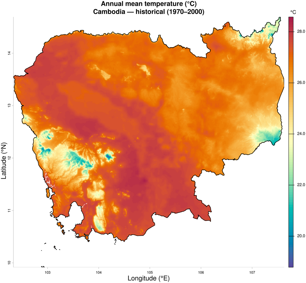

2. Mean annual precipitation — historical baseline (1970–2000)

Process:

Read in the precipitation GeoTIFF (12 monthly layers, each the 1970–2000 mean total for that month, in mm)
Calculate mean annual precipitation by summing the 12 monthly layers

# ---------------------------------------------------------------------------
# Mean annual precipitation — historical (1970–2000)
# Output: Gridded mean annual precipitation map
# ---------------------------------------------------------------------------

# Read in historical data
hist_prec <- rast(file.path(out_dir_historical, "tile_34_wc2.1_30s_prec.tif"))

# Crop and mask to national boundary (adm0 read in setvariables chunk)
hist_prec_c <- mask(crop(hist_prec, adm0), adm0)

# Total annual precipitation — sum across the 12 monthly layers
prec_annual <- app(hist_prec_c, sum)


## Plot
# Save output as PNG
fname <- file.path(out_dir_graphics, "annual_mean_prec_historical")

png(paste0(fname, ".png"), width = 12, height = 10, units = "in", res = 300, type = "cairo")

plot(prec_annual,
  main = "Mean annual precipitation (mm)\nCambodia — historical (1970–2000)",
  col = hcl.colors(100, "YlGnBu", rev = TRUE),
  mar = c(5.1, 4.1, 4.1, 2.1),
  xlab = "Longitude (°E)",
  ylab = "Latitude (°N)",
  cex.main = 1.3,
  cex.lab = 1.3,
  plg = list(title = "mm"),
  box = FALSE
)

lines(adm0, col = "black", lwd = 1.5)

dev.off()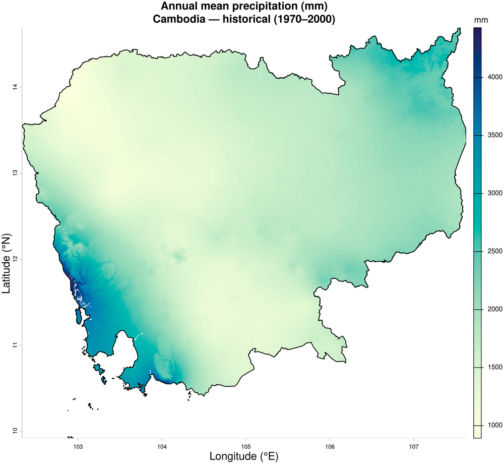

3. Mean annual temperature change — future (ensemble mean) minus historical

Temperature change maps are produced with a shared colour scale for cross-panel comparison.

Process (repeated for each SSP and time period):

Read in tmin and tmax for each of the 5 GCMs and crop/mask to the national boundary
Calculate mean annual temperature for each GCM, as the average of mean annual tmin and tmax: output 5 separate layers
Stack the 5 layers with rast(gcm_tmean_layers)
Take the mean across the 5 GCMs with app(…, mean): output single ensemble-mean layer
Subtract the historical mean annual temperature (tmean_annual): output anomaly map

# ---------------------------------------------------------------------------
# Mean annual temperature change — 2x2 grid (SSP x Year)
# Future ensemble mean minus historical
# Output: Spatial anomaly panel map
# ---------------------------------------------------------------------------

# Calculate all anomalies and store as list
temp_anomalies <- list()

for (ssp in ssps) {
  for (year in years) {
    key <- paste0(ssp, "_", year)
    message("Temperature change: ", ssp, " ", year)

    # Ensemble mean future tmean across GCMs
    gcm_tmean_layers <- list()
    for (g in gcms) {
      tmin <- rast(file.path(out_dir_future, sprintf("wc2.1_30s_tmin_%s_ssp%s_%s_tile-34.tif", g, ssp, year)))
      tmax <- rast(file.path(out_dir_future, sprintf("wc2.1_30s_tmax_%s_ssp%s_%s_tile-34.tif", g, ssp, year)))
      tmin_c <- mask(crop(tmin, adm0), adm0)
      tmax_c <- mask(crop(tmax, adm0), adm0)
      gcm_tmean_layers[[g]] <- (app(tmin_c, mean) + app(tmax_c, mean)) / 2
    }
    fut_tmean_annual <- app(rast(gcm_tmean_layers), mean)

    # Store anomaly
    temp_anomalies[[key]] <- fut_tmean_annual - tmean_annual
  }
}

## Common colour scale across all SSP/period panels (min to max)
temp_anom_range <- range(sapply(temp_anomalies, minmax))
print(temp_anom_range)


## Plot 2x2 grid with shared colour scale and national mean annotation
fname <- file.path(out_dir_graphics, "annual_temp_anomaly_2x2")

png(paste0(fname, ".png"), width = 12, height = 10, units = "in", res = 300, type = "cairo")

par(mfrow = c(2, 2))

for (ssp in ssps) {
  for (year in years) {
    key <- paste0(ssp, "_", year)
    ssp_label <- ifelse(ssp == "245", "SSP2-4.5", "SSP5-8.5")
    title <- paste0("Mean annual temperature change (°C)\n", ssp_label, " ", year, " relative to 1970–2000")
    mean_val <- as.numeric(global(temp_anomalies[[key]], mean, na.rm = TRUE))

    plot(temp_anomalies[[key]],
      main = title,
      mar = c(3.1, 3.1, 3.1, 5.1),
      col = hcl.colors(100, "YlOrRd", rev = TRUE),
      range = temp_anom_range,
      xlab = "Longitude (°E)",
      ylab = "Latitude (°N)",
      cex.main = 1.0,
      cex.lab = 1.0,
      legend = TRUE,
      box = FALSE
    )

    lines(adm0, col = "black", lwd = 1.5)

    # National mean annotation (sign added automatically)
    mtext(paste0("National mean: ", sprintf("%+.2f", mean_val), "°C"),
      side = 3, line = 0, cex = 0.8, font = 2
    )
  }
}

dev.off()


## Check actual mean anomaly values for each panel
# for (key in names(temp_anomalies)) {
#   cat(key, ":", round(as.numeric(global(temp_anomalies[[key]], mean, na.rm = TRUE)), 3), "°C\n")
# }

# 245_2041-2060 : 1.724 °C
# 245_2061-2080 : 2.232 °C
# 585_2041-2060 : 2.103 °C
# 585_2061-2080 : 3.239 °C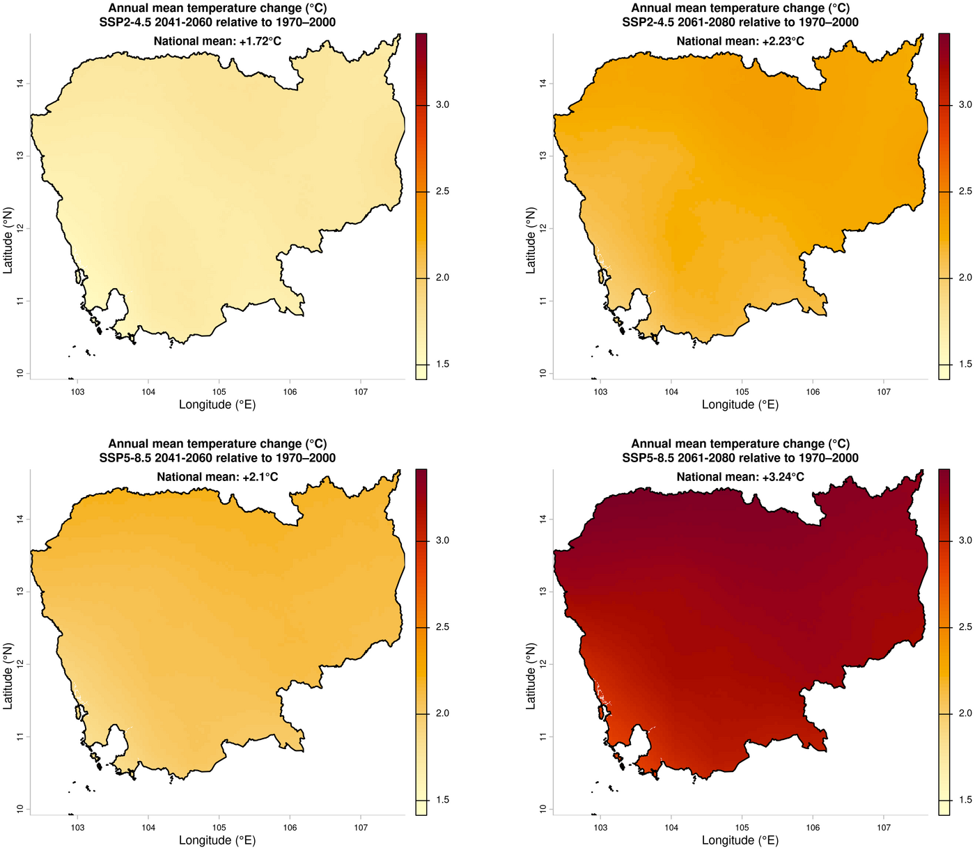

4. Mean annual precipitation change — ensemble mean relative to 1970–2000 (%)

Process (repeated for each SSP and time period):

Read in precipitation for each of the 5 GCMs (12 monthly layers each) and crop/mask to the national boundary
Calculate mean annual precipitation for each GCM by summing the 12 monthly layers with app(…, sum): output 5 separate layers
Stack the 5 layers with rast(gcm_prec_layers)
Take the mean across the 5 GCMs with app(…, mean): output single ensemble-mean layer
Calculate percentage change from the historical mean annual precipitation (prec_annual): ((future − historical) / historical) × 100

# ---------------------------------------------------------------------------
# Mean annual precipitation change — 2x2 grid (SSP x Year)
# Future ensemble mean vs. historical, as percentage change
# Output: Spatial anomaly panel map
# ---------------------------------------------------------------------------

# Calculate all anomalies and store as list
prec_anomalies <- list()
fut_prec_list <- list() 

for (ssp in ssps) {
  for (year in years) {
    key <- paste0(ssp, "_", year)
    message("Precipitation change: ", ssp, " ", year)

    # Ensemble mean future total annual precipitation across GCMs
    gcm_prec_layers <- list()
    for (g in gcms) {
      prec <- rast(file.path(out_dir_future, sprintf("wc2.1_30s_prec_%s_ssp%s_%s_tile-34.tif", g, ssp, year)))
      prec_c <- mask(crop(prec, adm0), adm0)
      gcm_prec_layers[[g]] <- app(prec_c, sum)
    }
    fut_prec_annual <- app(rast(gcm_prec_layers), mean)
    fut_prec_list[[key]] <- fut_prec_annual 

    # Store percentage change
    prec_anomalies[[key]] <- ((fut_prec_annual - prec_annual) / prec_annual) * 100
  }
}

## Common symmetric colour scale centred on zero (diverging palette)
prec_anom_abs_max <- max(abs(sapply(prec_anomalies, minmax)))
prec_anom_range <- c(-prec_anom_abs_max, prec_anom_abs_max)
print(prec_anom_range)


## Plot 2x2 grid with shared colour scale and national mean annotation
# Historical national mean (same baseline for all panels)
hist_nat <- as.numeric(global(prec_annual, mean, na.rm = TRUE))

fname <- file.path(out_dir_graphics, "annual_prec_anomaly_2x2")

png(paste0(fname, ".png"), width = 12, height = 10, units = "in", res = 300, type = "cairo")

par(mfrow = c(2, 2))

for (ssp in ssps) {
  for (year in years) {
    key <- paste0(ssp, "_", year)
    ssp_label <- ifelse(ssp == "245", "SSP2-4.5", "SSP5-8.5")
    title <- paste0("Mean annual precipitation change (%)\n", ssp_label, " ", year, " relative to 1970–2000")
    fut_nat <- as.numeric(global(fut_prec_list[[key]], mean, na.rm = TRUE))
    mean_val <- (fut_nat - hist_nat) / hist_nat * 100

    plot(prec_anomalies[[key]],
      main = title,
      mar = c(3.1, 3.1, 3.1, 5.1),
      col = hcl.colors(100, "BrBG"),
      range = prec_anom_range,
      xlab = "Longitude (°E)",
      ylab = "Latitude (°N)",
      cex.main = 1.0,
      cex.lab = 1.0,
      plg = list(title = "%"),
      box = FALSE
    )

    lines(adm0, col = "black", lwd = 1.5)

    # National mean annotation (sign added automatically)
    mtext(paste0("National mean: ", sprintf("%+.1f", mean_val), "%"),
      side = 3, line = 0, cex = 0.8, font = 2
    )
  }
}

dev.off()

# Check anomaly values:
# for (key in names(prec_anomalies)) {
#   cat(key, ":", round(as.numeric(minmax(prec_anomalies[[key]])), 2), "\n")
# }

5. Mean annual temperature change by GCM

Process (repeated for each SSP and time period):

Read in tmin and tmax for each of the 5 GCMs and crop/mask to the national boundary
Calculate each GCM’s national mean annual temperature, as the average of mean annual tmin and tmax across all pixels: output one value per GCM
Subtract the historical national mean annual temperature (from tmean_annual): output one anomaly per GCM
Plot each GCM’s anomaly, the range across GCMs, and the ensemble mean (the unweighted average of the 5 GCMs)

# ---------------------------------------------------------------------------
# Mean annual temperature change by GCM (national scalars)
# Model ensemble spread plot: GCM spread per SSP and time period
# ---------------------------------------------------------------------------

# Historical national mean baseline (tmean_annual from historical section)
hist_tmean_national <- as.numeric(global(tmean_annual, mean, na.rm = TRUE))

# Calculate mean annual temperature anomaly per GCM/SSP/year
gcm_temp_anomalies <- data.frame()

for (ssp in ssps) {
  for (year in years) {
    message("GCM temperature changes: ", ssp, " ", year)

    for (g in gcms) {
      tmin <- rast(file.path(out_dir_future, sprintf("wc2.1_30s_tmin_%s_ssp%s_%s_tile-34.tif", g, ssp, year)))
      tmax <- rast(file.path(out_dir_future, sprintf("wc2.1_30s_tmax_%s_ssp%s_%s_tile-34.tif", g, ssp, year)))
      tmin_c <- mask(crop(tmin, adm0), adm0)
      tmax_c <- mask(crop(tmax, adm0), adm0)

      gcm_tmean_national <- (as.numeric(global(app(tmin_c, mean), mean, na.rm = TRUE)) +
        as.numeric(global(app(tmax_c, mean), mean, na.rm = TRUE))) / 2

      gcm_temp_anomalies <- rbind(gcm_temp_anomalies, data.frame(
        gcm = g, ssp = ssp, year = year,
        temp_anomaly = gcm_tmean_national - hist_tmean_national
      ))
    }
  }
}


## Set up plot
# One group (row) per SSP/period combination, in loop order
groups <- unique(gcm_temp_anomalies[, c("ssp", "year")])
n_groups <- nrow(groups)
group_labels <- paste0(
  ifelse(groups$ssp == "245", "SSP2-4.5", "SSP5-8.5"), "  ",
  gsub("-", "–", groups$year)
)

all_vals <- gcm_temp_anomalies$temp_anomaly
xlim <- c(min(0, floor(min(all_vals) * 2) / 2), ceiling(max(all_vals) * 2) / 2)
ylim <- c(0.5, n_groups + 1)

ssp_cols <- c("245" = "#EAB139", "585" = "#980002")
gcm_pch <- setNames(c(16, 17, 15, 18, 8), gcms)


## Plot
fname <- file.path(out_dir_graphics, "annual_mean_temp_anomaly_gcm")
png(paste0(fname, ".png"), width = 10, height = 6, units = "in", res = 300, type = "cairo")
par(mar = c(4, 9, 4, 2), mgp = c(2.5, 0.5, 0))

plot(NA,
  xlim = xlim,
  ylim = ylim,
  xlab = "Temperature change (°C) relative to 1970–2000",
  ylab = "",
  yaxt = "n",
  main = "Mean annual temperature change by GCM\nCambodia — future projections",
  bty = "n",
  cex.main = 0.9
)

# Grid lines and zero reference
abline(v = seq(xlim[1], xlim[2], by = 0.5), col = "grey90", lty = 1, lwd = 0.8)
abline(v = 0, col = "grey30", lty = 2, lwd = 1.5)

# Plot dots, ranges, and means per group
for (i in seq_len(n_groups)) {
  this_group <- gcm_temp_anomalies[gcm_temp_anomalies$ssp == groups$ssp[i] &
    gcm_temp_anomalies$year == groups$year[i], ]
  vals <- setNames(this_group$temp_anomaly, this_group$gcm)
  col <- ssp_cols[[groups$ssp[i]]]
  ens_mean <- mean(vals)

  # Range bar
  segments(min(vals), i, max(vals), i, col = adjustcolor(col, alpha.f = 0.4), lwd = 3)

  # Ensemble mean — vertical line
  segments(ens_mean, i - 0.2, ens_mean, i + 0.2, col = col, lwd = 3)

  # Ensemble mean value above the vertical line (sign added automatically)
  text(ens_mean, i + 0.35,
    labels = paste0(sprintf("%+.2f", ens_mean), "°C"),
    col = col,
    cex = 0.75,
    font = 2
  )

  # Individual GCM points
  points(vals, rep(i, length(vals)), pch = gcm_pch[names(vals)], col = col, cex = 1.2)
}

# Y axis labels
axis(2, at = 1:n_groups, labels = group_labels, las = 1, cex.axis = 0.85, tcl = 0)

# Legend for GCMs (pch 124 = "|" for the ensemble mean line)
legend("bottomright",
  legend = c(gcms, "Ensemble mean"),
  pch = c(gcm_pch, 124),
  pt.cex = c(rep(1, length(gcms)), 1.4),
  col = "grey40",
  bty = "n",
  cex = 0.75,
  title = "CMIP6 projections",
  title.font = 2
)

dev.off()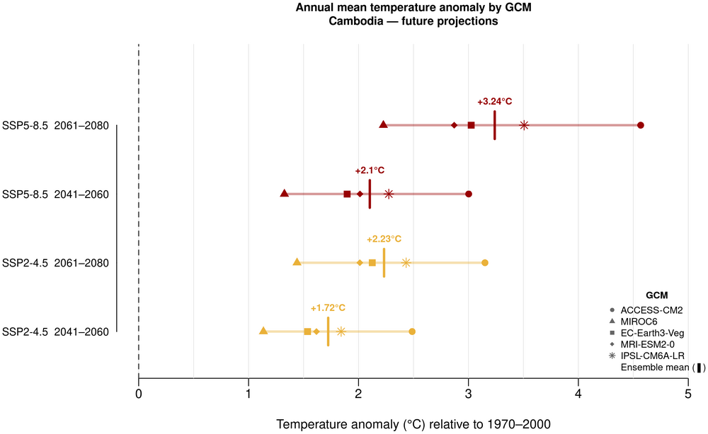

6. Mean annual precipitation change by GCM

Process (repeated for each SSP and time period):

Read in precipitation for each of the 5 GCMs (12 monthly layers each) and crop/mask to the national boundary
Calculate each GCM’s national mean annual precipitation: sum the 12 monthly layers, then average across all pixels. Output: one value per GCM
Calculate the percentage change from the historical national mean annual precipitation (from prec_annual): one value per GCM
Plot each GCM’s change, the range across GCMs, and the ensemble mean (the unweighted average of the 5 GCMs)

# ---------------------------------------------------------------------------
# Mean annual precipitation change by GCM (national scalars)
# Model ensemble spread plot: GCM spread per SSP and time period
# ---------------------------------------------------------------------------

# Historical national mean baseline (prec_annual from historical section)
hist_prec_national <- as.numeric(global(prec_annual, mean, na.rm = TRUE))

# Calculate annual precipitation anomaly (%) per GCM/SSP/year
gcm_prec_anomalies <- data.frame()

for (ssp in ssps) {
  for (year in years) {
    message("GCM precipitation changes: ", ssp, " ", year)

    for (g in gcms) {
      prec <- rast(file.path(out_dir_future, sprintf("wc2.1_30s_prec_%s_ssp%s_%s_tile-34.tif", g, ssp, year)))
      prec_c <- mask(crop(prec, adm0), adm0)

      gcm_prec_national <- as.numeric(global(app(prec_c, sum), mean, na.rm = TRUE))

      gcm_prec_anomalies <- rbind(gcm_prec_anomalies, data.frame(
        gcm = g, ssp = ssp, year = year,
        prec_anomaly_pct = ((gcm_prec_national - hist_prec_national) / hist_prec_national) * 100
      ))
    }
  }
}


## Set up plot
# One group (row) per SSP/period combination, in loop order
groups <- unique(gcm_prec_anomalies[, c("ssp", "year")])
n_groups <- nrow(groups)
group_labels <- paste0(
  ifelse(groups$ssp == "245", "SSP2-4.5", "SSP5-8.5"), "  ",
  gsub("-", "–", groups$year)
)

# x range always includes zero so the reference line is visible
all_vals <- gcm_prec_anomalies$prec_anomaly_pct
xlim <- c(min(0, floor(min(all_vals)) - 1), max(0, ceiling(max(all_vals)) + 1))
ylim <- c(0.5, n_groups + 1)

ssp_cols <- c("245" = "#EAB139", "585" = "#980002")
gcm_pch <- setNames(c(16, 17, 15, 18, 8), gcms)


## Plot
fname <- file.path(out_dir_graphics, "annual_mean_prec_anomaly_gcm")

png(paste0(fname, ".png"), width = 10, height = 6, units = "in", res = 300, type = "cairo")
par(mar = c(4, 9, 4, 2), mgp = c(2.5, 0.5, 0))

plot(NA,
  xlim = xlim,
  ylim = ylim,
  xlab = "Precipitation change (%) relative to 1970–2000",
  ylab = "",
  yaxt = "n",
  main = "Mean annual precipitation change by GCM\nCambodia — future projections",
  bty = "n",
  cex.main = 0.9
)

# Grid lines every 2% (aligned to even numbers) and zero reference
abline(v = seq(2 * floor(xlim[1] / 2), xlim[2], by = 2), col = "grey90", lty = 1, lwd = 0.8)
abline(v = 0, col = "grey30", lty = 2, lwd = 1.5)

# Plot dots, ranges, and means per group
for (i in seq_len(n_groups)) {
  this_group <- gcm_prec_anomalies[gcm_prec_anomalies$ssp == groups$ssp[i] &
    gcm_prec_anomalies$year == groups$year[i], ]
  vals <- setNames(this_group$prec_anomaly_pct, this_group$gcm)
  col <- ssp_cols[[groups$ssp[i]]]
  ens_mean <- mean(vals)

  # Range bar
  segments(min(vals), i, max(vals), i, col = adjustcolor(col, alpha.f = 0.4), lwd = 3)

  # Ensemble mean — vertical line
  segments(ens_mean, i - 0.2, ens_mean, i + 0.2, col = col, lwd = 3)

  # Ensemble mean value above the vertical line (sign added automatically)
  text(ens_mean, i + 0.35,
    labels = paste0(sprintf("%+.1f", ens_mean), "%"),
    col = col,
    cex = 0.75,
    font = 2
  )

  # Individual GCM points
  points(vals, rep(i, length(vals)), pch = gcm_pch[names(vals)], col = col, cex = 1.2)
}

# Y axis labels
axis(2, at = 1:n_groups, labels = group_labels, las = 1, cex.axis = 0.85, tcl = 0)

# Legend for GCMs (pch 124 = "|" for the ensemble mean line)
legend("bottomright",
  legend = c(gcms, "Ensemble mean"),
  pch = c(gcm_pch, 124),
  pt.cex = c(rep(1, length(gcms)), 1.4),
  col = "grey40",
  bty = "n",
  cex = 0.75,
  title = "CMIP6 projections",
  title.font = 2
)

dev.off()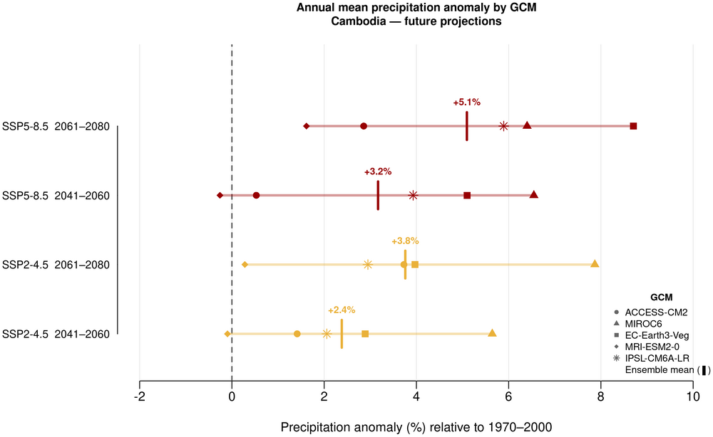

Monthly graphics

The following can be applied to generate monthly graphics for any region of the world.

1. Mean monthly temperature and precipitation — historical baseline (1970–2000)

Process:

Calculate national mean monthly values from the cropped historical rasters (hist_tmin_c, hist_tmax_c, hist_prec_c): one value per month for minimum, maximum and mean temperature and for precipitation
Plot monthly precipitation as bars (left axis) and mean temperature as a line (right axis), with temperature rescaled onto the precipitation axis

# ---------------------------------------------------------------------------
# Mean monthly precipitation and temperature — historical (1970–2000)
# Output: Climate chart (precipitation bars, temperature line)
# Uses hist_tmin_c, hist_tmax_c, hist_prec_c from the historical sections
# ---------------------------------------------------------------------------

month_labels <- c("Jan", "Feb", "Mar", "Apr", "May", "Jun", "Jul", "Aug", "Sep", "Oct", "Nov", "Dec")

# Monthly national spatial means
monthly_hist <- data.frame(
  month = month_labels,
  tmin = as.numeric(global(hist_tmin_c, mean, na.rm = TRUE)$mean),
  tmax = as.numeric(global(hist_tmax_c, mean, na.rm = TRUE)$mean),
  prec = as.numeric(global(hist_prec_c, mean, na.rm = TRUE)$mean)
)
monthly_hist$tmean <- (monthly_hist$tmin + monthly_hist$tmax) / 2

# Scaling: map temperature onto precipitation axis
# Scale temp to fit within precipitation axis range
prec_max <- max(monthly_hist$prec) * 1.15
temp_min <- floor(min(monthly_hist$tmean)) - 1
temp_max <- ceiling(max(monthly_hist$tmean)) + 1
temp_range <- temp_max - temp_min

# Linear scaling function: temp -> prec axis
temp_to_prec <- function(t) (t - temp_min) / temp_range * prec_max


## Plot
fname <- file.path(out_dir_graphics, "monthly_mean_prec_temp_historical")

png(paste0(fname, ".png"), width = 8, height = 6, units = "in", res = 300, type = "cairo")

par(mar = c(5, 4, 4, 4), mgp = c(3, 0.3, 0))

# Precipitation bars
bp <- barplot(monthly_hist$prec,
  names.arg = monthly_hist$month,
  col = adjustcolor("steelblue", alpha.f = 0.7),
  border = NA,
  ylim = c(0, prec_max),
  ylab = "",
  xlab = "",
  main = "Mean monthly precipitation and temperature\nCambodia — historical (1970–2000)",
  las = 1,
  cex.names = 0.9,
  cex.axis = 0.8,
  tcl = -0.2
)

# Left y-axis title
mtext("Mean monthly precipitation (mm)", side = 2, line = 1.8, cex = 0.8)

# Temperature line (scaled to precipitation axis)
lines(bp, temp_to_prec(monthly_hist$tmean), col = "firebrick", lwd = 2.5)
points(bp, temp_to_prec(monthly_hist$tmean), col = "firebrick", pch = 16, cex = 0.8)

# Right y-axis: temperature
temp_ticks <- seq(temp_min, temp_max, by = 2)
axis(4,
  at = temp_to_prec(temp_ticks),
  labels = temp_ticks,
  las = 1,
  cex.axis = 0.8,
  tcl = -0.2
)
mtext("Mean monthly temperature (°C)", side = 4, line = 1.8, cex = 0.8)

# Precipitation value labels (offset scales with the axis)
text(bp, monthly_hist$prec + prec_max * 0.025,
  labels = round(monthly_hist$prec, 0),
  cex = 0.75,
  col = "grey30"
)

# Annual total annotation
annual_total <- sum(monthly_hist$prec)
mtext(paste0("Mean annual precipitation: ", round(annual_total, 0), " mm"),
  side = 1, line = 2.5, cex = 0.85, font = 2
)

# Legend
legend("topleft",
  legend = c("Mean monthly precipitation", "Mean monthly temperature"),
  fill = c(adjustcolor("steelblue", alpha.f = 0.7), NA),
  border = c(NA, NA),
  lwd = c(NA, 2.5),
  col = c(NA, "firebrick"),
  pch = c(NA, 16),
  bty = "n",
  cex = 0.8
)

dev.off()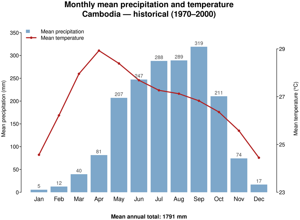

2. Mean monthly temperature — historical and future projections

Historical line + SSP2-4.5 and SSP5-8.5 ribbons (GCM spread) in two panels for 2041–2060 and 2061–2080.

Process (repeated for each SSP and time period):

Read in tmin and tmax for each of the 5 GCMs and crop/mask to the national boundary
Calculate each GCM’s national mean monthly temperature, (tmin + tmax) / 2: output 12 values per GCM
Summarise across the 5 GCMs for each month: ensemble mean (dashed line) and minimum–maximum range (ribbon)
Plot against the historical mean monthly temperature from section 1 (black line)

# ---------------------------------------------------------------------------
# Mean monthly temperature — ensemble range plot
# Historical + SSP2-4.5 and SSP5-8.5 ribbons (GCM spread)
# Two panels: 2041–2060 and 2061–2080
# Uses monthly_hist and month_labels from section 1 (mean monthly precipitation and temperature)
# ---------------------------------------------------------------------------

# Calculate monthly ensemble mean, min and max across GCMs per SSP/period
monthly_future_temp <- data.frame()

for (ssp in ssps) {
  for (year in years) {
    message("Monthly temperature: ", ssp, " ", year)

    # One row per GCM, one column per month
    gcm_monthly <- list()
    for (g in gcms) {
      tmin <- rast(file.path(out_dir_future, sprintf("wc2.1_30s_tmin_%s_ssp%s_%s_tile-34.tif", g, ssp, year)))
      tmax <- rast(file.path(out_dir_future, sprintf("wc2.1_30s_tmax_%s_ssp%s_%s_tile-34.tif", g, ssp, year)))
      tmin_c <- mask(crop(tmin, adm0), adm0)
      tmax_c <- mask(crop(tmax, adm0), adm0)
      tmin_m <- as.numeric(global(tmin_c, mean, na.rm = TRUE)$mean)
      tmax_m <- as.numeric(global(tmax_c, mean, na.rm = TRUE)$mean)
      gcm_monthly[[g]] <- (tmin_m + tmax_m) / 2
    }
    gcm_mat <- do.call(rbind, gcm_monthly)

    # Summarise across GCMs for each month
    monthly_future_temp <- rbind(monthly_future_temp, data.frame(
      month = month_labels, ssp = ssp, year = year,
      tmean_mean = colMeans(gcm_mat),
      tmean_min = apply(gcm_mat, 2, min),
      tmean_max = apply(gcm_mat, 2, max)
    ))
  }
}


## Set up plot
mon <- 1:12
ssp_labels <- c("245" = "SSP2-4.5", "585" = "SSP5-8.5")
ssp_cols <- c("245" = "#EAB139", "585" = "#980002")

# Shared y-axis across both panels so periods are directly comparable
ylim <- range(monthly_hist$tmean, monthly_future_temp$tmean_min, monthly_future_temp$tmean_max) + c(-0.5, 0.5)

# Legend entries generated from ssps (mean line + range ribbon per SSP)
legend_labels <- c("Historical (1970–2000)", as.vector(rbind(
  paste(ssp_labels[ssps], "ensemble mean"),
  paste(ssp_labels[ssps], "GCM range")
)))
legend_cols <- c("black", as.vector(rbind(
  ssp_cols[ssps],
  adjustcolor(ssp_cols[ssps], alpha.f = 0.2)
)))
legend_lwd <- c(2.5, rep(c(2, 8), length(ssps)))
legend_lty <- c(1, rep(c(2, 1), length(ssps)))


## Plot
fname <- file.path(out_dir_graphics, "monthly_mean_temperature_hist_future")

png(paste0(fname, ".png"), width = 12, height = 6, units = "in", res = 300, type = "cairo")

par(mfrow = c(1, 2), mar = c(4, 3.5, 4, 2), mgp = c(1.8, 0.5, 0))

for (year in years) {
  # Set up empty plot
  plot(mon, monthly_hist$tmean,
    type = "n",
    xlab = "",
    ylab = "Mean monthly temperature (°C)",
    xaxt = "n",
    yaxt = "n",
    ylim = ylim,
    main = paste0("Mean monthly temperature\nCambodia — historical and future projections (", gsub("-", "–", year), ")"),
    bty = "n",
    cex.main = 1.0
  )

  axis(1, at = mon, labels = month_labels, cex.axis = 0.85, tcl = -0.2)
  axis(2, las = 1, cex.axis = 0.8)

  # GCM range ribbons (drawn first so lines sit on top)
  for (ssp in ssps) {
    this_ssp <- monthly_future_temp[monthly_future_temp$ssp == ssp & monthly_future_temp$year == year, ]
    polygon(c(mon, rev(mon)),
      c(this_ssp$tmean_max, rev(this_ssp$tmean_min)),
      col = adjustcolor(ssp_cols[[ssp]], alpha.f = 0.2),
      border = NA
    )
  }

  # Ensemble mean lines
  for (ssp in ssps) {
    this_ssp <- monthly_future_temp[monthly_future_temp$ssp == ssp & monthly_future_temp$year == year, ]
    lines(mon, this_ssp$tmean_mean, col = ssp_cols[[ssp]], lwd = 2, lty = 2)
  }

  # Historical line
  lines(mon, monthly_hist$tmean, col = "black", lwd = 2.5)

  # Legend (inset 10% from left, 2% from bottom)
  legend("bottomleft",
    inset = c(0.1, 0.02),
    legend = legend_labels,
    col = legend_cols,
    lwd = legend_lwd,
    lty = legend_lty,
    bty = "n",
    cex = 0.75
  )
}

dev.off()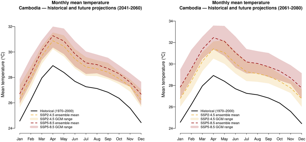

3. Mean monthly precipitation — historical and future projections

Historical line + SSP2-4.5 and SSP5-8.5 ribbons (GCM spread) in two panels for 2041–2060 and 2061–2080.

Process (repeated for each SSP and time period):

Read in precipitation for each of the 5 GCMs (12 monthly layers each) and crop/mask to the national boundary
Calculate each GCM’s national mean monthly precipitation: output 12 values per GCM
Summarise across the 5 GCMs for each month: ensemble mean (dashed line) and minimum–maximum range (ribbon)
Plot against the historical mean monthly precipitation from section 1 (black line)

# ---------------------------------------------------------------------------
# Mean monthly precipitation — ensemble range plot
# Historical + SSP2-4.5 and SSP5-8.5 ribbons (GCM spread)
# Two panels: 2041–2060 and 2061–2080
# Uses monthly_hist and month_labels from section 1 (mean monthly precipitation and temperature)
# ---------------------------------------------------------------------------

# Calculate monthly ensemble mean, min and max across GCMs per SSP/period
monthly_future_prec <- data.frame()

for (ssp in ssps) {
  for (year in years) {
    message("Monthly precipitation: ", ssp, " ", year)

    # One row per GCM, one column per month
    gcm_monthly <- list()
    for (g in gcms) {
      prec <- rast(file.path(out_dir_future, sprintf("wc2.1_30s_prec_%s_ssp%s_%s_tile-34.tif", g, ssp, year)))
      prec_c <- mask(crop(prec, adm0), adm0)
      gcm_monthly[[g]] <- as.numeric(global(prec_c, mean, na.rm = TRUE)$mean)
    }
    gcm_mat <- do.call(rbind, gcm_monthly)

    # Summarise across GCMs for each month
    monthly_future_prec <- rbind(monthly_future_prec, data.frame(
      month = month_labels, ssp = ssp, year = year,
      prec_mean = colMeans(gcm_mat),
      prec_min = apply(gcm_mat, 2, min),
      prec_max = apply(gcm_mat, 2, max)
    ))
  }
}


## Set up plot
mon <- 1:12
ssp_labels <- c("245" = "SSP2-4.5", "585" = "SSP5-8.5")
ssp_cols <- c("245" = "#EAB139", "585" = "#980002")

# Shared y-axis across both panels; lower limit floored at 0 mm
prec_vals <- c(monthly_hist$prec, monthly_future_prec$prec_min, monthly_future_prec$prec_max)
ylim <- c(max(0, min(prec_vals) - 10), max(prec_vals) + 20)

# Legend entries generated from ssps (mean line + range ribbon per SSP)
legend_labels <- c("Historical (1970–2000)", as.vector(rbind(
  paste(ssp_labels[ssps], "ensemble mean"),
  paste(ssp_labels[ssps], "GCM range")
)))
legend_cols <- c("black", as.vector(rbind(
  ssp_cols[ssps],
  adjustcolor(ssp_cols[ssps], alpha.f = 0.2)
)))
legend_lwd <- c(2.5, rep(c(2, 8), length(ssps)))
legend_lty <- c(1, rep(c(2, 1), length(ssps)))


## Plot
fname <- file.path(out_dir_graphics, "monthly_mean_prec_hist_future")

png(paste0(fname, ".png"), width = 12, height = 6, units = "in", res = 300, type = "cairo")

par(mfrow = c(1, 2), mar = c(4, 3.5, 4, 2), mgp = c(1.8, 0.5, 0))

for (year in years) {
  # Set up empty plot
  plot(mon, monthly_hist$prec,
    type = "n",
    xlab = "",
    ylab = "Mean monthly precipitation (mm)",
    xaxt = "n",
    yaxt = "n",
    ylim = ylim,
    main = paste0("Mean monthly precipitation\nCambodia — historical and future projections (", gsub("-", "–", year), ")"),
    bty = "n",
    cex.main = 1.0
  )

  axis(1, at = mon, labels = month_labels, cex.axis = 0.85, tcl = -0.2)
  axis(2, las = 1, cex.axis = 0.8)

  # GCM range ribbons (drawn first so lines sit on top)
  for (ssp in ssps) {
    this_ssp <- monthly_future_prec[monthly_future_prec$ssp == ssp & monthly_future_prec$year == year, ]
    polygon(c(mon, rev(mon)),
      c(this_ssp$prec_max, rev(this_ssp$prec_min)),
      col = adjustcolor(ssp_cols[[ssp]], alpha.f = 0.2),
      border = NA
    )
  }

  # Ensemble mean lines
  for (ssp in ssps) {
    this_ssp <- monthly_future_prec[monthly_future_prec$ssp == ssp & monthly_future_prec$year == year, ]
    lines(mon, this_ssp$prec_mean, col = ssp_cols[[ssp]], lwd = 2, lty = 2)
  }

  # Historical line
  lines(mon, monthly_hist$prec, col = "black", lwd = 2.5)

  # Legend (inset 10% from left, 2% from top)
  legend("topleft",
    inset = c(0.1, 0.02),
    legend = legend_labels,
    col = legend_cols,
    lwd = legend_lwd,
    lty = legend_lty,
    bty = "n",
    cex = 0.75
  )
}

dev.off()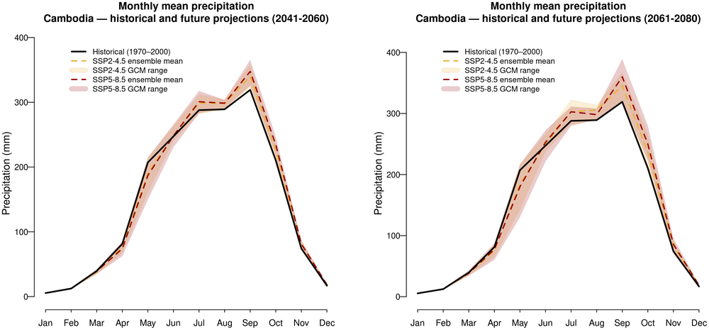

Seasonal maps and graphics

These outputs are tailored to Cambodia and rice cultivation. They use Cambodia’s monsoonal seasons: wet season May–November and dry season December–April (Chhinh & Millington, 2015). For other regions, change wet_months and dry_months (see above).

1. Wet-season precipitation change — ensemble mean relative to 1970–2000

Process (repeated for each SSP and time period):

Sum the historical wet-season months for each pixel to give historical wet-season precipitation
Read in precipitation for each of the 5 GCMs and crop/mask to the national boundary
Sum the wet-season months for each GCM: output 5 separate layers
Take the mean across the 5 GCMs with app(…, mean): output single ensemble-mean layer
Calculate percentage change from historical: ((future − historical) / historical) × 100

# ---------------------------------------------------------------------------
# Wet-season precipitation change (%) — 2x2 grid (SSP x Year)
# Future ensemble mean vs. historical (1970–2000)
# Wet season months set by wet_months as stated above
# Output: Spatial anomaly panel map
# ---------------------------------------------------------------------------

# Historical national mean wet-season precipitation (same baseline for all panels)
hist_prec_ws <- app(subset(hist_prec_c, wet_months), sum)
hist_ws_nat <- as.numeric(global(hist_prec_ws, mean, na.rm = TRUE))

# Calculate all anomalies and store as list
ws_prec_anomalies <- list()
fut_prec_ws_list <- list()

for (ssp in ssps) {
  for (year in years) {
    key <- paste0(ssp, "_", year)
    message("Wet-season precipitation change: ", ssp, " ", year)

    # Ensemble mean future wet-season total across GCMs
    gcm_prec_ws_layers <- list()
    for (g in gcms) {
      prec <- rast(file.path(out_dir_future, sprintf("wc2.1_30s_prec_%s_ssp%s_%s_tile-34.tif", g, ssp, year)))
      prec_c <- mask(crop(prec, adm0), adm0)
      gcm_prec_ws_layers[[g]] <- app(subset(prec_c, wet_months), sum)
    }
    fut_prec_ws <- app(rast(gcm_prec_ws_layers), mean)
    fut_prec_ws_list[[key]] <- fut_prec_ws

    # Store percentage change
    ws_prec_anomalies[[key]] <- ((fut_prec_ws - hist_prec_ws) / hist_prec_ws) * 100
  }
}

## Common symmetric colour scale centred on zero (diverging palette)
ws_prec_anom_abs_max <- max(abs(sapply(ws_prec_anomalies, minmax)))
ws_prec_anom_range <- c(-ws_prec_anom_abs_max, ws_prec_anom_abs_max)
print(ws_prec_anom_range)


## Plot 2x2 grid with shared colour scale and national mean annotation
fname <- file.path(out_dir_graphics, "wet_season_prec_change_2x2")

png(paste0(fname, ".png"), width = 12, height = 10, units = "in", res = 300, type = "cairo")

par(mfrow = c(2, 2))

for (ssp in ssps) {
  for (year in years) {
    key <- paste0(ssp, "_", year)
    ssp_label <- ifelse(ssp == "245", "SSP2-4.5", "SSP5-8.5")
    title <- paste0("Wet-season precipitation change (%)\n", ssp_label, " ", year, " relative to 1970–2000")
    fut_ws_nat <- as.numeric(global(fut_prec_ws_list[[key]], mean, na.rm = TRUE))
    mean_val <- (fut_ws_nat - hist_ws_nat) / hist_ws_nat * 100

    plot(ws_prec_anomalies[[key]],
      main = title,
      mar = c(3.1, 3.1, 3.1, 5.1),
      col = hcl.colors(100, "BrBG"),
      range = ws_prec_anom_range,
      xlab = "Longitude (°E)",
      ylab = "Latitude (°N)",
      cex.main = 1.0,
      cex.lab = 1.0,
      plg = list(title = "%"),
      box = FALSE
    )

    lines(adm0, col = "black", lwd = 1.5)

    # National mean annotation (sign added automatically)
    mtext(paste0("National mean: ", sprintf("%+.1f", mean_val), "%"),
      side = 3, line = 0, cex = 0.8, font = 2
    )
  }
}

dev.off()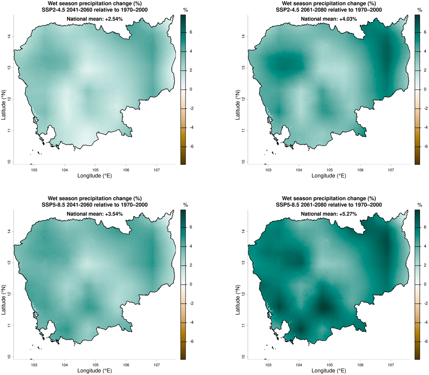

2. Dry-season precipitation change — ensemble mean relative to 1970–2000

Process (repeated for each SSP and time period):

Sum the historical dry-season months for each pixel to give historical dry-season precipitation
Read in precipitation for each of the 5 GCMs and crop/mask to the national boundary
Sum the dry-season months for each GCM: output 5 separate layers
Take the mean across the 5 GCMs with app(…, mean): output single ensemble-mean layer
Calculate percentage change from historical: ((future − historical) / historical) × 100

# ---------------------------------------------------------------------------
# Dry-season precipitation change (%) — 2x2 grid (SSP x Year)
# Future ensemble mean vs. historical (1970–2000)
# Dry season months set by dry_months (as above)
# Output: Spatial anomaly panel map
# ---------------------------------------------------------------------------

# Historical dry-season total precipitation per pixel
hist_prec_ds <- app(subset(hist_prec_c, dry_months), sum)

# Calculate all anomalies and store as list
ds_prec_anomalies <- list()
fut_prec_ds_list <- list()

for (ssp in ssps) {
  for (year in years) {
    key <- paste0(ssp, "_", year)
    message("Dry-season precipitation change: ", ssp, " ", year)

    # Ensemble mean future dry-season total across GCMs
    gcm_prec_ds_layers <- list()
    for (g in gcms) {
      prec <- rast(file.path(out_dir_future, sprintf("wc2.1_30s_prec_%s_ssp%s_%s_tile-34.tif", g, ssp, year)))
      prec_c <- mask(crop(prec, adm0), adm0)
      gcm_prec_ds_layers[[g]] <- app(subset(prec_c, dry_months), sum)
    }
    fut_prec_ds <- app(rast(gcm_prec_ds_layers), mean)
    fut_prec_ds_list[[key]] <- fut_prec_ds

    # Store percentage change
    ds_prec_anomalies[[key]] <- ((fut_prec_ds - hist_prec_ds) / hist_prec_ds) * 100
  }
}

## Common symmetric colour scale centred on zero (diverging palette)
ds_prec_anom_abs_max <- max(abs(sapply(ds_prec_anomalies, minmax)))
ds_prec_anom_range <- c(-ds_prec_anom_abs_max, ds_prec_anom_abs_max)
print(ds_prec_anom_range)

# Outlier check: compare 99th percentile with maximum of absolute change.
# If close, extremes are representative and the min/max scale is kept.
# ds_vals <- unlist(lapply(ds_prec_anomalies, function(r) values(r, na.rm = TRUE)))
# quantile(abs(ds_vals), c(0.5, 0.9, 0.99, 1))
# Result (2026-10-12): 99% = 6.33, max = 7.83 — min/max scale kept


## Plot 2x2 grid with shared colour scale and national mean annotation
# Historical national mean dry-season precipitation (same baseline for all panels)
hist_ds_nat <- as.numeric(global(hist_prec_ds, mean, na.rm = TRUE))

fname <- file.path(out_dir_graphics, "dry_season_prec_change_2x2")

png(paste0(fname, ".png"), width = 12, height = 10, units = "in", res = 300, type = "cairo")

par(mfrow = c(2, 2))

for (ssp in ssps) {
  for (year in years) {
    key <- paste0(ssp, "_", year)
    ssp_label <- ifelse(ssp == "245", "SSP2-4.5", "SSP5-8.5")
    title <- paste0("Dry-season precipitation change (%)\n", ssp_label, " ", year, " relative to 1970–2000")
    fut_ds_nat <- as.numeric(global(fut_prec_ds_list[[key]], mean, na.rm = TRUE))
    mean_val <- (fut_ds_nat - hist_ds_nat) / hist_ds_nat * 100

    plot(ds_prec_anomalies[[key]],
      main = title,
      mar = c(3.1, 3.1, 3.1, 5.1),
      col = hcl.colors(100, "BrBG"),
      range = ds_prec_anom_range,
      xlab = "Longitude (°E)",
      ylab = "Latitude (°N)",
      cex.main = 1.0,
      cex.lab = 1.0,
      plg = list(title = "%"),
      box = FALSE
    )

    lines(adm0, col = "black", lwd = 1.5)

    # National mean annotation: % change in national mean dry-season precipitation
    mtext(paste0("National mean: ", sprintf("%+.1f", mean_val), "%"),
      side = 3, line = 0, cex = 0.8, font = 2
    )
  }
}

dev.off()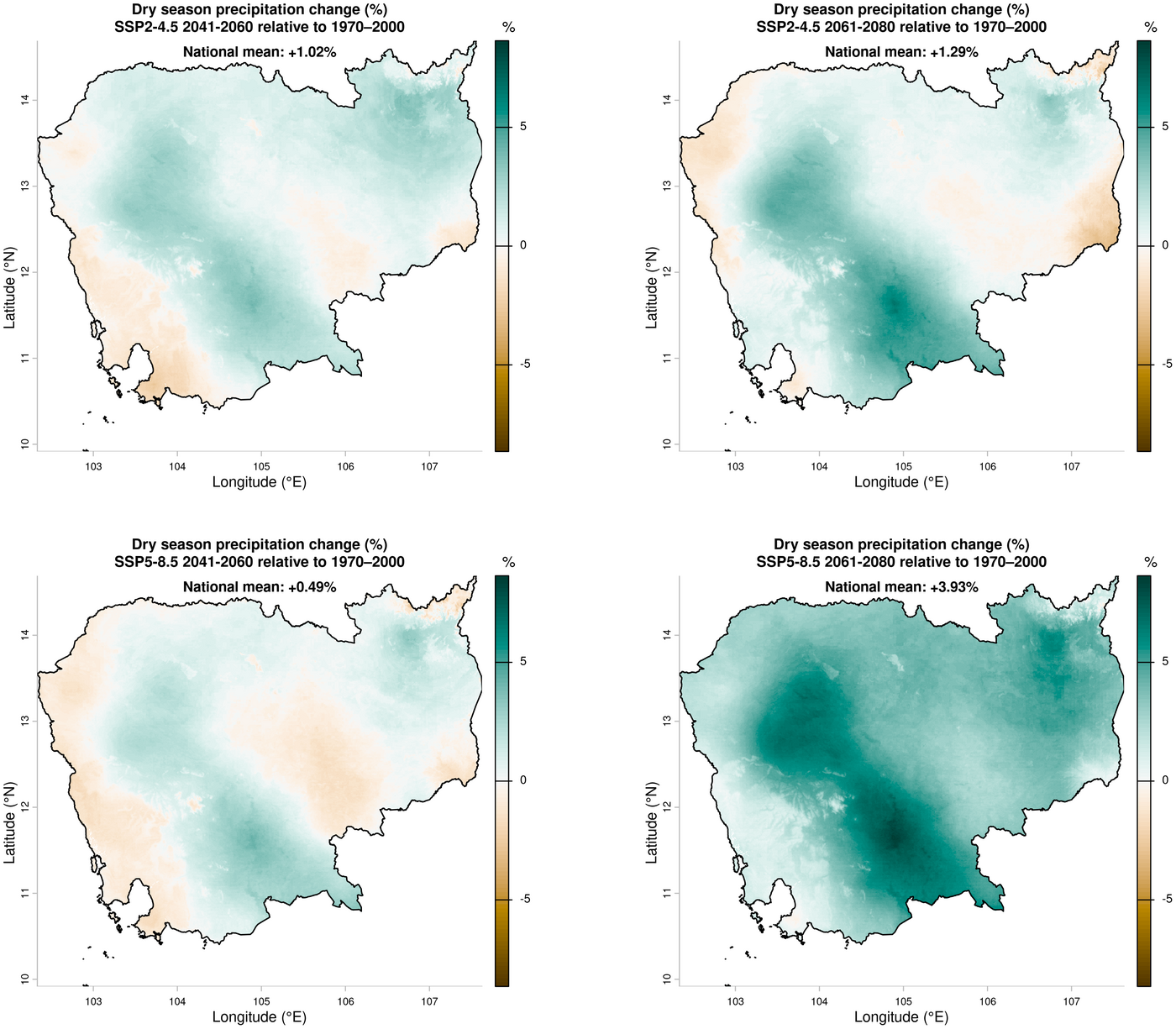

3. Dry-season mean temperature change — ensemble mean minus 1970–2000

Process (repeated for each SSP and time period):

Average the historical dry-season months of tmin and tmax for each pixel, then take their midpoint to give historical dry-season mean temperature
Read in tmin and tmax for each of the 5 GCMs and crop/mask to the national boundary
Calculate dry-season mean temperature for each GCM in the same way: output 5 separate layers
Take the mean across the 5 GCMs with app(…, mean): output single ensemble-mean layer
Subtract historical dry-season mean temperature: output change in °C

# ---------------------------------------------------------------------------
# Dry-season mean temperature change (°C) — 2x2 grid (SSP x Year)
# Future ensemble mean minus historical (1970–2000)
# Dry season months set by dry_months as above
# Output: Spatial anomaly panel map
# ---------------------------------------------------------------------------

# Historical dry-season mean temperature per pixel
hist_tmin_ds <- subset(hist_tmin_c, dry_months)
hist_tmax_ds <- subset(hist_tmax_c, dry_months)
hist_tmean_ds <- (app(hist_tmin_ds, mean) + app(hist_tmax_ds, mean)) / 2

# Calculate all anomalies and store as list
ds_temp_anomalies <- list()

for (ssp in ssps) {
  for (year in years) {
    key <- paste0(ssp, "_", year)
    message("Dry-season temperature change: ", ssp, " ", year)

    # Ensemble mean future dry-season tmean across GCMs
    gcm_tmean_ds_layers <- list()
    for (g in gcms) {
      tmin <- rast(file.path(out_dir_future, sprintf("wc2.1_30s_tmin_%s_ssp%s_%s_tile-34.tif", g, ssp, year)))
      tmax <- rast(file.path(out_dir_future, sprintf("wc2.1_30s_tmax_%s_ssp%s_%s_tile-34.tif", g, ssp, year)))
      tmin_c <- mask(crop(tmin, adm0), adm0)
      tmax_c <- mask(crop(tmax, adm0), adm0)
      tmin_ds <- subset(tmin_c, dry_months)
      tmax_ds <- subset(tmax_c, dry_months)
      gcm_tmean_ds_layers[[g]] <- (app(tmin_ds, mean) + app(tmax_ds, mean)) / 2
    }
    fut_tmean_ds <- app(rast(gcm_tmean_ds_layers), mean)

    # Store anomaly (absolute change in °C)
    ds_temp_anomalies[[key]] <- fut_tmean_ds - hist_tmean_ds
  }
}

## Common colour scale across all SSP/period panels (min to max)
ds_temp_anom_range <- range(sapply(ds_temp_anomalies, minmax))
print(ds_temp_anom_range)


## Plot 2x2 grid with shared colour scale and national mean annotation
fname <- file.path(out_dir_graphics, "dry_season_tmean_change_2x2")

png(paste0(fname, ".png"), width = 12, height = 10, units = "in", res = 300, type = "cairo")

par(mfrow = c(2, 2))

for (ssp in ssps) {
  for (year in years) {
    key <- paste0(ssp, "_", year)
    ssp_label <- ifelse(ssp == "245", "SSP2-4.5", "SSP5-8.5")
    title <- paste0("Dry-season mean temperature change (°C)\n", ssp_label, " ", year, " relative to 1970–2000")
    mean_val <- as.numeric(global(ds_temp_anomalies[[key]], mean, na.rm = TRUE))

    plot(ds_temp_anomalies[[key]],
      main = title,
      mar = c(3.1, 3.1, 3.1, 5.1),
      col = hcl.colors(100, "YlOrRd", rev = TRUE),
      range = ds_temp_anom_range,
      xlab = "Longitude (°E)",
      ylab = "Latitude (°N)",
      cex.main = 1.0,
      cex.lab = 1.0,
      plg = list(title = "°C"),
      box = FALSE
    )

    lines(adm0, col = "black", lwd = 1.5)

    # National mean annotation (sign added automatically)
    mtext(paste0("National mean: ", sprintf("%+.2f", mean_val), "°C"),
      side = 3, line = 0, cex = 0.8, font = 2
    )
  }
}

dev.off()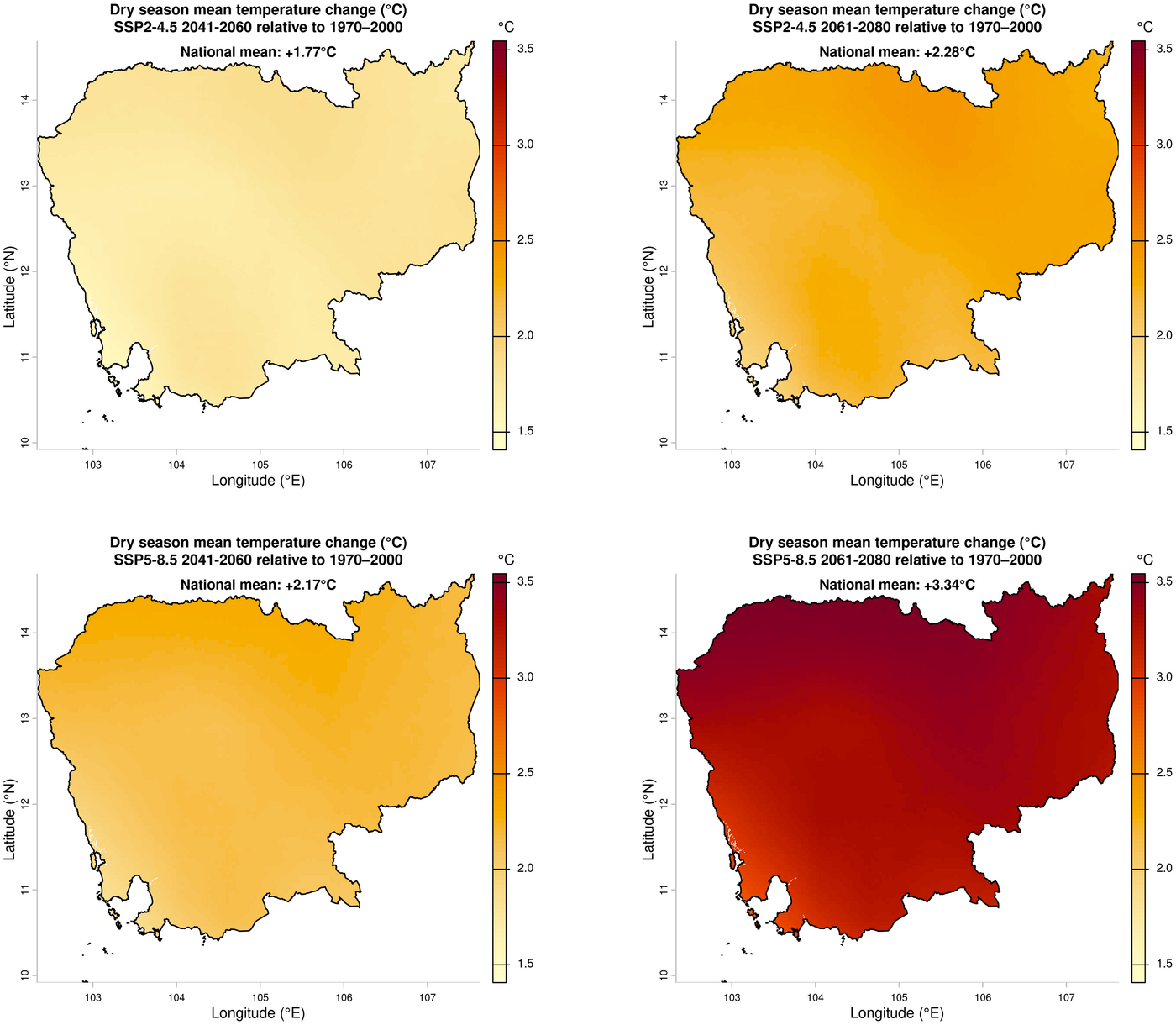

4. Mean monthly precipitation and monsoon periods — historical and future projections

Historical line + SSP2-4.5 and SSP5-8.5 ribbons (GCM spread) in two panels for 2041–2060 and 2061–2080, with the wet and dry seasons shaded and south-west monsoon onset and cessation marked.

Process:

Reuse the historical and future monthly precipitation calculated in the Monthly graphics section (section 3, mean monthly precipitation): no files are re-read
Shade the wet and dry seasons using wet_months and dry_months (see above)
Mark monsoon onset at the start of the first wet-season month and cessation at the end of the last

# ---------------------------------------------------------------------------
# Mean monthly precipitation with monsoon period overlay
# Historical + SSP2-4.5 and SSP5-8.5 ribbons (GCM spread)
# Wet/dry season shading and SW monsoon onset/cessation from
# wet_months and dry_months (as above)
# Two panels: 2041–2060 and 2061–2080
# Uses monthly_hist and month_labels (Monthly graphics section 1) and
# monthly_future_prec (Monthly graphics section 3)
# ---------------------------------------------------------------------------

## Set up plot
mon <- 1:12
ssp_labels <- c("245" = "SSP2-4.5", "585" = "SSP5-8.5")
ssp_cols <- c("245" = "#EAB139", "585" = "#980002")

# Shared y-axis across both panels; lower limit floored at 0 mm
prec_vals <- c(monthly_hist$prec, monthly_future_prec$prec_min, monthly_future_prec$prec_max)
ylim <- c(max(0, min(prec_vals) - 10), max(prec_vals) + 20)

# Season of each month, grouped into contiguous runs for shading
# (dry season wraps the year end, so it appears as two runs: Jan-Apr, Dec)
season <- ifelse(mon %in% wet_months, "Wet", ifelse(mon %in% dry_months, "Dry", NA))
season_runs <- rle(season)
run_ends <- cumsum(season_runs$lengths)
run_starts <- run_ends - season_runs$lengths + 1
season_fill <- c("Wet" = adjustcolor("steelblue", alpha.f = 0.06), "Dry" = adjustcolor("tan3", alpha.f = 0.06))
season_text <- c("Wet" = "steelblue", "Dry" = "tan4")

# Monsoon onset/cessation at the wet-season boundaries
# (assumes the wet season falls within one calendar year, as May-Nov does)
onset_x <- min(wet_months) - 0.5
cessation_x <- max(wet_months) + 0.5

# Legend entries generated from ssps (mean line + range ribbon per SSP)
legend_labels <- c("Historical (1970–2000)", as.vector(rbind(
  paste(ssp_labels[ssps], "ensemble mean"),
  paste(ssp_labels[ssps], "GCM range")
)))
legend_cols <- c("black", as.vector(rbind(
  ssp_cols[ssps],
  adjustcolor(ssp_cols[ssps], alpha.f = 0.2)
)))
legend_lwd <- c(2.5, rep(c(2, 8), length(ssps)))
legend_lty <- c(1, rep(c(2, 1), length(ssps)))


## Plot
fname <- file.path(out_dir_graphics, "prec_seasonal_monsoon")

png(paste0(fname, ".png"), width = 12, height = 7, units = "in", res = 300, type = "cairo")

par(mfrow = c(1, 2), mar = c(5, 4.5, 4, 2), mgp = c(2.5, 0.5, 0))

for (year in years) {
  # Empty plot
  plot(mon, monthly_hist$prec,
    type = "n",
    xlab = "",
    ylab = "Mean monthly precipitation (mm)",
    xaxt = "n",
    yaxt = "n",
    ylim = ylim,
    main = paste0("Mean monthly precipitation and monsoon periods\nCambodia — historical and future projections (", gsub("-", "–", year), ")"),
    bty = "n",
    cex.main = 0.9
  )

  # Wet/dry season background shading and labels
  for (r in seq_along(season_runs$values)) {
    s <- season_runs$values[r]
    if (is.na(s)) next
    rect(run_starts[r] - 0.5, ylim[1], run_ends[r] + 0.5, ylim[2], col = season_fill[[s]], border = NA)
    mtext(s, side = 3, at = (run_starts[r] + run_ends[r]) / 2, line = -2.5, cex = 0.7, col = season_text[[s]], font = 3)
  }

  # Onset/cessation reference lines and annotations
  abline(v = c(onset_x, cessation_x), col = "steelblue", lty = 3, lwd = 1.2)
  label_y <- ylim[2] - diff(ylim) * 0.04
  text(onset_x, label_y, paste0("Onset\n(", month_labels[min(wet_months)], ")"), cex = 0.65, col = "steelblue")
  text(cessation_x, label_y, paste0("Cessation\n(", month_labels[max(wet_months)], ")"), cex = 0.65, col = "steelblue")

  axis(1, at = mon, labels = month_labels, cex.axis = 0.85, tcl = -0.2)
  axis(2, las = 1, cex.axis = 0.8)

  # GCM range ribbons (drawn first so lines sit on top)
  for (ssp in ssps) {
    this_ssp <- monthly_future_prec[monthly_future_prec$ssp == ssp & monthly_future_prec$year == year, ]
    polygon(c(mon, rev(mon)),
      c(this_ssp$prec_max, rev(this_ssp$prec_min)),
      col = adjustcolor(ssp_cols[[ssp]], alpha.f = 0.2),
      border = NA
    )
  }

  # Ensemble mean lines
  for (ssp in ssps) {
    this_ssp <- monthly_future_prec[monthly_future_prec$ssp == ssp & monthly_future_prec$year == year, ]
    lines(mon, this_ssp$prec_mean, col = ssp_cols[[ssp]], lwd = 2, lty = 2)
  }

  # Historical line
  lines(mon, monthly_hist$prec, col = "black", lwd = 2.5)

  # Legend (inset 2% from left, 12% from top, below the season labels)
  legend("topleft",
    inset = c(0.02, 0.12),
    legend = legend_labels,
    col = legend_cols,
    lwd = legend_lwd,
    lty = legend_lty,
    bty = "n",
    cex = 0.72
  )
}

dev.off()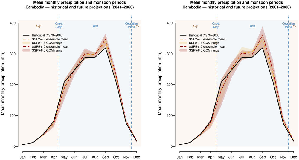

5. Mean monthly maximum temperature and 35°C threshold — historical and future projections

Historical line + SSP2-4.5 and SSP5-8.5 ribbons (GCM spread) in two panels for 2041–2060 and 2061–2080, against a 35°C threshold. Triangles mark months where the upper end of the SSP5-8.5 GCM range reaches the threshold.

Process (repeated for each SSP and time period):

Read in tmax for each of the 5 GCMs and crop/mask to the national boundary
Calculate each GCM’s national mean monthly maximum temperature: output 12 values per GCM
Summarise across the 5 GCMs for each month: ensemble mean (dashed line) and minimum–maximum range (ribbon)
Plot against the historical mean monthly maximum temperature from Monthly graphics section 1 (black line)

The 35°C threshold is indicative. Heat stress thresholds for rice refer to daily maximum temperatures during flowering, whereas this plot shows monthly means averaged across the country. Individual days, and hotter locations, will exceed these values, so the plot understates how often 35°C is reached.

# ---------------------------------------------------------------------------
# Mean monthly maximum temperature — ensemble range plot
# Historical + SSP2-4.5 and SSP5-8.5 ribbons (GCM spread), with
# 35°C threshold line
# Two panels: 2041–2060 and 2061–2080
# Uses monthly_hist and month_labels from Monthly graphics section 1
# ---------------------------------------------------------------------------

# Threshold for mean monthly maximum temperature (°C)
tmax_threshold <- 35

# Calculate monthly tmax ensemble mean, min and max across GCMs per SSP/period
monthly_future_tmax <- data.frame()

for (ssp in ssps) {
  for (year in years) {
    message("Monthly maximum temperature: ", ssp, " ", year)

    # One row per GCM, one column per month
    gcm_monthly <- list()
    for (g in gcms) {
      tmax <- rast(file.path(out_dir_future, sprintf("wc2.1_30s_tmax_%s_ssp%s_%s_tile-34.tif", g, ssp, year)))
      tmax_c <- mask(crop(tmax, adm0), adm0)
      gcm_monthly[[g]] <- as.numeric(global(tmax_c, mean, na.rm = TRUE)$mean)
    }
    gcm_mat <- do.call(rbind, gcm_monthly)

    # Summarise across GCMs for each month
    monthly_future_tmax <- rbind(monthly_future_tmax, data.frame(
      month = month_labels, ssp = ssp, year = year,
      tmax_mean = colMeans(gcm_mat),
      tmax_min = apply(gcm_mat, 2, min),
      tmax_max = apply(gcm_mat, 2, max)
    ))
  }
}


## Set up plot
mon <- 1:12
ssp_labels <- c("245" = "SSP2-4.5", "585" = "SSP5-8.5")
ssp_cols <- c("245" = "#EAB139", "585" = "#980002")

# Highest-emission scenario, used for the exceedance markers
ssp_high <- ssps[length(ssps)]

# Shared y-axis across both panels, always including the threshold
ylim <- range(monthly_hist$tmax, monthly_future_tmax$tmax_min, monthly_future_tmax$tmax_max, tmax_threshold) + c(-0.5, 1)

# Legend entries generated from ssps, plus threshold line and exceedance marker
legend_labels <- c(
  "Historical (1970–2000)",
  as.vector(rbind(paste(ssp_labels[ssps], "ensemble mean"), paste(ssp_labels[ssps], "GCM range"))),
  paste0(tmax_threshold, "°C threshold"),
  paste0(ssp_labels[ssp_high], " GCM range reaches ", tmax_threshold, "°C")
)
legend_cols <- c(
  "black",
  as.vector(rbind(ssp_cols[ssps], adjustcolor(ssp_cols[ssps], alpha.f = 0.2))),
  "firebrick", "firebrick"
)
legend_lwd <- c(2.5, rep(c(2, 8), length(ssps)), 1.5, NA)
legend_lty <- c(1, rep(c(2, 1), length(ssps)), 2, NA)
legend_pch <- c(rep(NA, 1 + 2 * length(ssps)), NA, 17)


## Plot
fname <- file.path(out_dir_graphics, "monthly_tmax_hist_future")

png(paste0(fname, ".png"), width = 12, height = 6, units = "in", res = 300, type = "cairo")

par(mfrow = c(1, 2), mar = c(4, 4, 4, 2), mgp = c(2.5, 0.5, 0))

for (year in years) {
  # Empty plot
  plot(mon, monthly_hist$tmax,
    type = "n",
    xlab = "",
    ylab = "Mean monthly maximum temperature (°C)",
    xaxt = "n",
    yaxt = "n",
    ylim = ylim,
    main = paste0("Mean monthly maximum temperature\nCambodia — historical and future projections (", gsub("-", "–", year), ")"),
    bty = "n",
    cex.main = 0.9
  )
  
   # Subtitle: what the triangles show
  mtext(paste0("Triangles: months where the ", ssp_labels[ssp_high], " GCM range reaches ", tmax_threshold, "°C"),
    side = 3, line = 0, cex = 0.7, font = 3
  )

  axis(1, at = mon, labels = month_labels, cex.axis = 0.85, tcl = -0.2)
  axis(2, las = 1, cex.axis = 0.8)

  # Threshold line and label
  abline(h = tmax_threshold, col = "firebrick", lty = 2, lwd = 1.5)
  text(12, tmax_threshold,
    labels = paste0(tmax_threshold, "°C threshold"),
    col = "firebrick",
    cex = 0.7,
    adj = c(1, -0.5)
  )

  # GCM range ribbons (drawn first so lines sit on top)
  for (ssp in ssps) {
    this_ssp <- monthly_future_tmax[monthly_future_tmax$ssp == ssp & monthly_future_tmax$year == year, ]
    polygon(c(mon, rev(mon)),
      c(this_ssp$tmax_max, rev(this_ssp$tmax_min)),
      col = adjustcolor(ssp_cols[[ssp]], alpha.f = 0.2),
      border = NA
    )
  }

  # Ensemble mean lines
  for (ssp in ssps) {
    this_ssp <- monthly_future_tmax[monthly_future_tmax$ssp == ssp & monthly_future_tmax$year == year, ]
    lines(mon, this_ssp$tmax_mean, col = ssp_cols[[ssp]], lwd = 2, lty = 2)
  }

  # Historical line
  lines(mon, monthly_hist$tmax, col = "black", lwd = 2.5)

  # Mark months where the highest-emission GCM range reaches the threshold
  this_high <- monthly_future_tmax[monthly_future_tmax$ssp == ssp_high & monthly_future_tmax$year == year, ]
  exceed <- which(this_high$tmax_max >= tmax_threshold)
  if (length(exceed) > 0) {
    points(exceed, rep(tmax_threshold, length(exceed)), pch = 17, col = "firebrick", cex = 1.0)
  }

  # Legend (inset 12% from left, 2% from bottom)
  legend("bottomleft",
    inset = c(0.12, 0.02),
    legend = legend_labels,
    col = legend_cols,
    lwd = legend_lwd,
    lty = legend_lty,
    pch = legend_pch,
    bty = "n",
    cex = 0.72
  )
}

dev.off()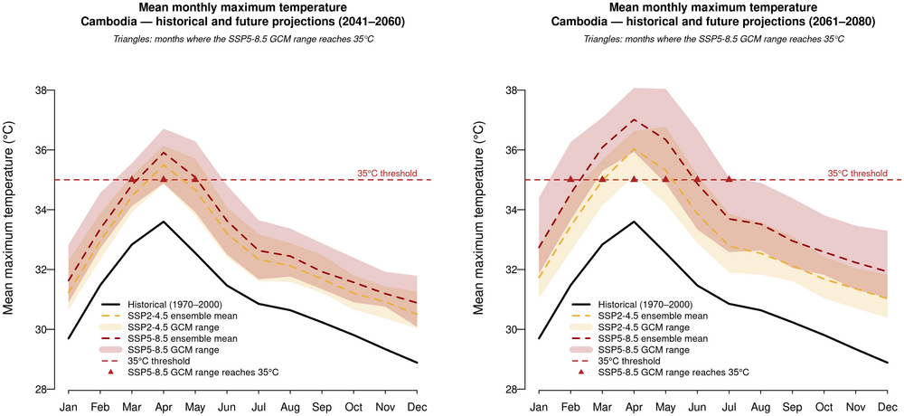

Code

The full Quarto document can be downloaded from GitHub: https://github.com/richardtc/transferable-climate-profile

References

Chhinh, N., & Millington, A. (2015). Drought monitoring for rice production in Cambodia. Climate, 3(4), 792–811. https://doi.org/10.3390/cli3040792

Introduction

Prerequisites

Download GCM data: five models, two scenarios and two future periods

Download historical data

Download future projections

Annual maps and graphics

1. Mean annual temperature — historical baseline (1970–2000)

2. Mean annual precipitation — historical baseline (1970–2000)

3. Mean annual temperature change — future (ensemble mean) minus historical

4. Mean annual precipitation change — ensemble mean relative to 1970–2000 (%)

5. Mean annual temperature change by GCM

6. Mean annual precipitation change by GCM

Monthly graphics

1. Mean monthly temperature and precipitation — historical baseline (1970–2000)

2. Mean monthly temperature — historical and future projections

3. Mean monthly precipitation — historical and future projections

Seasonal maps and graphics

1. Wet-season precipitation change — ensemble mean relative to 1970–2000

2. Dry-season precipitation change — ensemble mean relative to 1970–2000

3. Dry-season mean temperature change — ensemble mean minus 1970–2000

4. Mean monthly precipitation and monsoon periods — historical and future projections

5. Mean monthly maximum temperature and 35°C threshold — historical and future projections

Code

References

Footnotes